Auxiliary Uses of Decision Trees:
Optimal Binning of Continuous Variables Using Decision Trees in SAS E-Guide
Introduction
An interval or continuous variable has infinite number of discrete values, such as the operator age or vehicle length. Also, these continuous variables, very frequently, have missing observations, outliers, repeated observations etc. that makes inefficient try to use these variables as a continuous variable during the modeling process.
It is very frequent also, that several variables are sparsely populated (greater than90 percent missing values), so we need to address missing values. Normally, we would use imputation methodology to replace missing values with statistically generated values. However, we theorize that such a high number of imputed missing values could skew the distribution of the original variables and bias our predictions. Instead, we address missing values by optimal binning. We consider dropping the highly missing variables, but, given the high number of missing values, we realized these might have a significant effect in a predictive model.
For numeric variables with missing values, we decide to create “optimal bins.” Optimal bins are created by converting a numeric variable into a categorical variable in such a way that its relationship with the target is maximized in terms of a purity measure, such as chi-square, Gini coefficient, F-Test, variance reduction, etc.
Identifying factor levels can be arbitrary, judgmental, or optimality driven. Decision trees are transparent, intuitive, non-parametric, and robust to influential values, outliers, and missing values; therefore, they can be used to find optimal bins, or factor levels.
Example
The target variable in our model is the Loss Ratio. A typical risk factor is the operator age. In the following graph we can see the relationship between the Loss Ratio and the operator age:
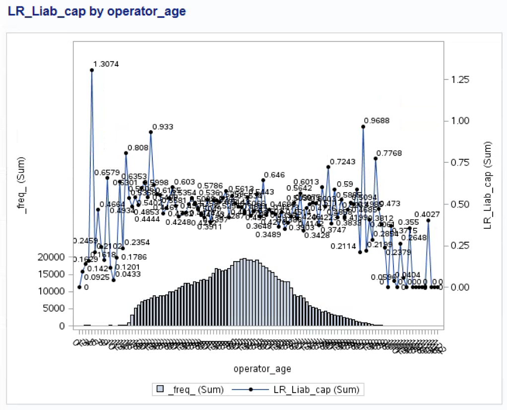
In the above plot, the operator age variable has been discretized in many levels. It is not easy to find a clear relationship.
We would like to see a clear pattern using an optimal criterion. We can use decision trees to accomplish this task in an optimal way.
Implementation Using the HPSPLIT Procedure
We can use the new HPSPLIT procedure in SAS STAT 13.2 (THE current version of SAS) to create decision trees in SAS Enterprise Guide 7.1 (the current version of SAS Enterprise Guide). Therefore, we don’t need to leave the SAS Enterprise Guide context in order to create our decision trees in SAS Enterprise Miner. When we use a decision tree to create an optimal binning for a continuous variable, several other decisions must also be made during this process. - How many leaves should have the decision tree? - What is the maximum tree depth? - What should the level of significance for factor splits be? - What splitting criterion should be used? - Should there be a minimum number of members in a node (policies or claims) to create a split? - How Specifies how to handle missing values in an input variable?
The answers to the above question are the following: - The level are conditioned by the number of observations in our dataset. In a typical context of data mining with several million of observation a subjective criteria many times applied as starting point is 16. - The maxims tree depth should be one. Here we are using a decision tree such an auxiliary tool in our modeling process, therefore, we would like only to collapse the variable in few levels. - The significant level for this kind of exercises usually is large, that is 0.1. - We should prevent post-pruning. - The splitting criteria in the context of this example with at continuous target should be Variance or F-Test. - The number of minimum observations in a node should be a credible exposure. - The HPSPLIT is able to handle the missing values based on three options: - BRANCH requests that missing values be assigned to their own branch. - POPULARITY requests that missing values be assigned to the most popular, or largest, branch. -SIMILARITY requests that missing values be assigned to the branch they are most similar to (using the chi-square or F test criterion)
An implementation of the above criteria using the HPSPLIT procedure in the context of our above example is the following SAS code:
ods graphics on;
proc hpsplit data=Auto_DS_BT maxdepth=1 missing = branch /*intervalbins= 10*/ maxbranch=8  leafsize=5000 alpha=0.1;
criterion variance; /*default for interval target VARIANCE or FTEST */
prune none;
target LR_liab_cap / level = int;
input operator_age / level = int;
output nodestats=stat;
run;

title 'Tree visualization';
proc print data=stat noobs;
run;
Where:
- The dataset is Auto_DS_BT
- The maximum depth of the tree to be grown equals one
- The MAXBRANCH option specifies the maximum number of children per node in the tree. PROC HPSPLIT tries to create this number of children unless it is impossible (for example, if a split variable does not have enough levels). The default is the number of target levels. The maximum number of branches in our example is 9
- The minimum number of polices in each and every leaf is 5000, a credible amount. This option specifies the minimum number of observations that a split must contain in the training data set in order for the split to be considered. By default, LEAFSIZE=1.
- The split criterion used is the F-Test. By default, CRITERION = variance
- The alpha option specify the maximum p-value for a split to be considered, in this case 0.1. By default is 0.3. This option is only considered if you specify the FTEST criterion
- The prune option is not used
- The target variable is LR_Liab_cap. We used the level = int option to indicate that the target variable is continuous
- The explanatory variable is OPERATOR_AGE. We used the level = int option to indicate that the explanatory variable is interval
- The output of the decision tree calculation is the SAS dataset called STAT
- The option for missing handle is not implemented in the current STAT product. Therefore, by default the criteria is POPULARITY. In the example we selected the BRANCH method in order to create an specific group for the missing observations
Finally, I used the PRINT procedure to visualize the output:

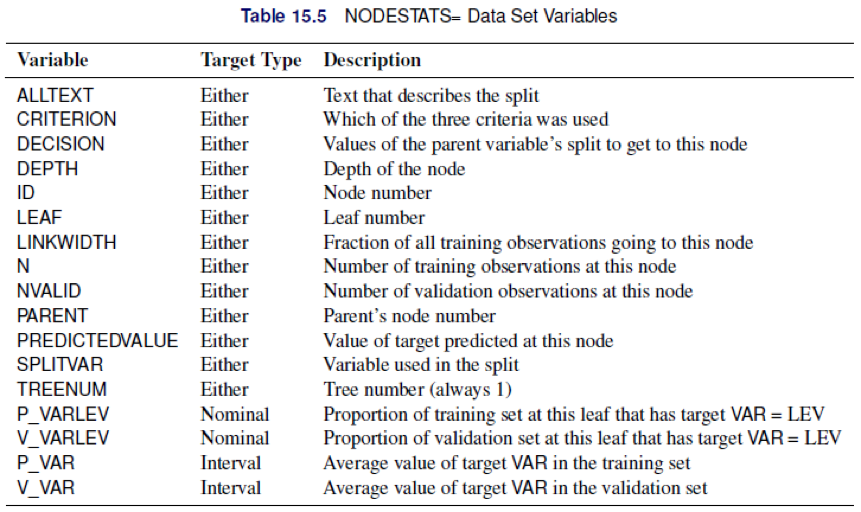
Thankfully to the decision tree we have a derived new variable that groups the OPERATOR_AGE in an optimal way:
     if operator_age eq .  then operator_age_grp = "00: Miss.";
else if operator_age lt 27 then operator_age_grp = "01: Lt 27";
else if operator_age lt 56 then operator_age_grp = "02: 28-56";
else if operator_age lt 64 then operator_age_grp = "03: 57-64";
else if operator_age lt 71 then operator_age_grp = "04: 65-71";
else if operator_age lt 74 then operator_age_grp = "05: 71-74";
else if operator_age lt 80 then operator_age_grp = "06: 74-80";
else if operator_age ge 80 then operator_age_grp = "07: Gt 80";
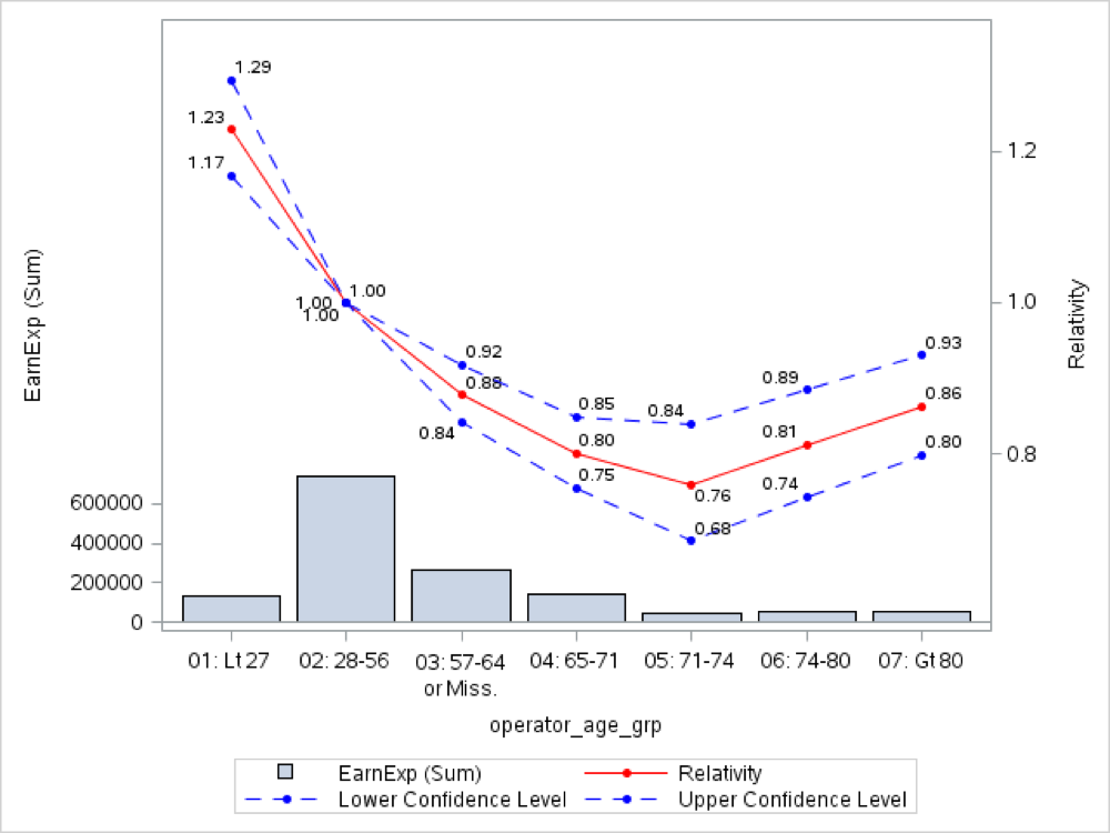
The relativities for the OPERATOR_AGE_GRP variable in a multivariate model are (training dataset):
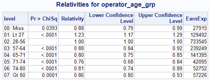
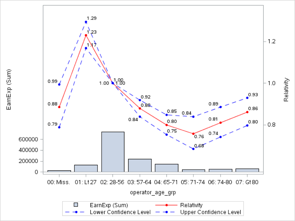
Now the characteristic ‘U’ shape relationship for the driver age arise clearly. Also, it is clear that the missing observations should be collapsed with the drivers between 57 and 65 years.

Summary
- The new HPSPLIT can be used as an auxiliary tool during the modeling process creating an optimal binning for interval or continuous variables.
- Identifying factor levels can be arbitrary, judgmental, or optimality driven. Decision trees are transparent, intuitive, non-parametric, and robust to influential values, outliers, and missing values.
- The process is very quickly and you don’t need to leave the SAS E-Guide context to use SAS Enterprise Miner
- Because the HPSPLIT is a high performance (HP) procedure, the tree fitting takes only few seconds. Therefore, it is really easy to use a macro to apply this procedure to other variables.
Appendix: Regression Trees, Partition Criteria and Heteroscedasticity
There are two splitting criteria used in regression tress:
- The first criterion is based on impurity function of a node. When the target distribution is continuous, the sample variance is the obvious measure of impurity.
- The second criterion is based on a statistical test for one-way ANOVA, the F-Test.
Some differences between the two above criteria:
- The F test is better than (sample) variance reduction as it has P-value adjustment number of branches.
- F test is relatively robust to departures from normality assumption
- However, F test is sensitive to departures from non-constant variance
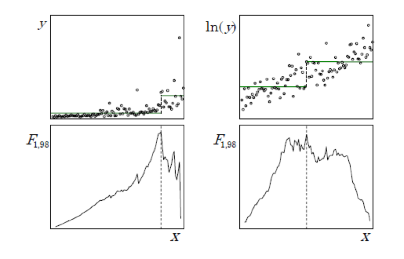
The F test has many optimal properties when the distribution of the target is independently and normally distributed with constant variance. The F test is relatively robust to departures from the normality assumption. However, variance heterogeneity (heteroscedasticity) can have disastrous effects. For example, the F test is too liberal (overstates the significance of the effect) when small nodes have larger variance. Consider the common case of a nonnegative target with variance increasing with the mean. Using the F test as the splitting criterion will tend to favor small splits of the largest values. Decision trees are usually regarded as robust and nonparametric. However, regression trees are not robust to heteroscedasticity. Like classical regression models, finding a suitable variance stabilizing transformation can improve the model. For example, apply a logarithm or a squared root transformation to the target variable. A typical context where a logarithm transformation is useful happens when the severity is the target variable.
Appendix: The INTERVALBINS option in the HPSPLIT Statement
There is an option of the HPSPLIT statement called INTERVALIBINS that devoted to create a specific number of bins in an interval variable. Here we have a description of this option.
INTERVALBINS=number specifies the number of bins for interval variables. By default, INTERVALBINS=100.
This option only works if we don’t use the MAXDEPTH=1 option and obviously the MAXBRANCH=8 option.
ods graphics on;
proc hpsplit data=Auto_DS_BT /*maxdepth=1*/ missing = branch intervalbins=8 /*maxbranch=8*/  leafsize=5000 alpha=0.1;
criterion variance; /*default for interval target VARIANCE or FTEST */
prune none;
target LR_liab_cap / level = int;
input operator_age / level = int;
output nodestats=stat;
run;

title 'Tree visualization';
proc print data=stat noobs;
run;
Without the MAXDEPTH option equal to one, we get also 8 levels, but, in this case, the decision tree has 4 depth levels. In our current version of SAS STAT 13.2, a graphical decision tree easy to interpret, is not implement. Only in the new SAS STAT 14.1 we can see in SAS E-Guide something like this:
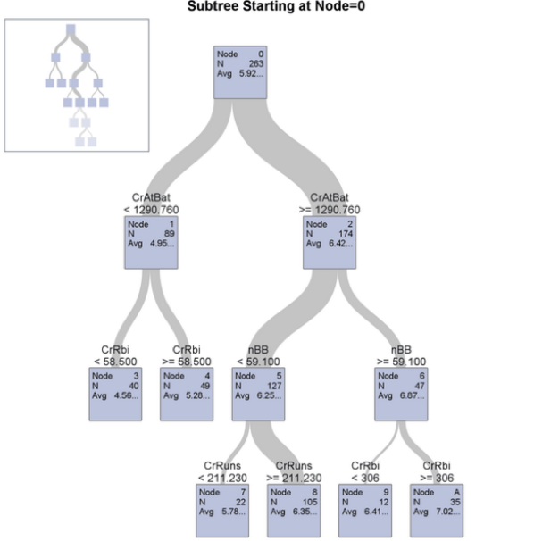
Therefore, we get a relatively more complex table that is not obvious how interpret without experience with decision trees:

Note that, the above tree shape graph and many other option are available at SAS Enterprise Miner. Here, we only try to show how to use SAS E-Guide to fit a basic decision tree instead to use SAS E-Miner.
References
- De Ville, Barry, and Padraic Neville. 2013. Decision Trees for Analytics Using SAS® Enterprise Miner. Cary, NC: SAS Institute Inc.
- The Anti-Curse: Creating an Extension to SAS® Enterprise Miner™ Using PROC ARBORETUM Andrew Cathie, SAS Institute (NZ) Ltd, Auckland, New Zealand
- Decision Tree Modeling Course Notes was developed by William J.E. Potts and revised by Lorne Rothman. Technical review was provided by Bob Lucas and Michael J. Patetta. 2006 by SAS Institute Inc. Chapter 4 – Auxiliary Uses of Trees. Section 4.3. - Collapsing Levels
- SAS/STAT® 13.2 User’s Guide High-Performance Procedures - Chapter 15. The HPSPLIT Procedure
- SAS Enterprise Miner 13.2 High Performance Data Mining Nodes Help
- Machine Learning With SAS® Enterprise Miner™ How a Team of SAS® Modelers Created and Determined a Champion Model to Predict Churn Using KDD Cup Data
- Ratemaking Using SAS® Enterprise Miner™: An Application Stud Billie Anderson, SAS Institute Inc., Cary, NC